How to train your MAML: A step by step approach

Antreas Antoniou, Harrison Edwards, Amos Storkey (2018) How to train your MAML. (arXiv:1810.09502).
Preface
Enter meta-learning, a universe where computational models, composed by multiple levels of learning abstractions, can improve their own ability to learn by learning some or all of their own building blocks (e.g. optimizers, loss functions, initializations, learning rates, updated functions, architectures etc.) through experience over a large number of tasks. Meta-learning or as often referred to learning to learn is achieved by abstracting learning into two or more levels. The inner-most levels acquire task-specific knowledge (e.g. fine-tuning a model on a new dataset) , whereas the outer-most level acquires across-task knowledge (e.g. learning to transfer between tasks more efficiently). If the models in the inner-most levels make use of components with learnable parameters, the outer-most optimization process can meta-learn the parameters of such components, thus enabling automatic learning of inner-loop components.
Few-shot learning is a perfect example of a problem-area where meta-learning can be used to effectively meta-learn a solution. Using meta-learning, one can formulate and train systems that can very quickly learn from a small training set (i.e. a support set), containing only 1-5 samples from each class, such that it can generalize strongly on a corresponding small validation set (i.e. a target set). The constraints in this instance are that the model will only have access to very few data-points from each class, and the target metric is the target set’s cross-entropy error.
Meta-learning can be achieved through a variety of learning paradigms. The most effective, as of the time of writing this, are supervised learning, reinforcement learning and genetic algorithms. Both reinforcement learning and genetic algorithms have been demonstrated to be very computationally expensive, often requiring hundreds of GPU hours for a single experiment. However, gradient-based, end-to-end differentiable supervised meta-learning schemes, such as Meta-learner LSTM and Model Agnostic Meta-Learning (MAML), can be run on a single GPU, within 12-24 hours.
Gradient-based, end-to-end differentiable meta-learning presents an incredible opportunity for efficient and effective meta-learning. However, methods from this family of meta-learning are currently in their infancy, often suffering from a variety of issues.
For example, MAML’s inner loop SGD optimizer can outperform the Meta-learner LSTM method, which has parameterized its update rule as an LSTM that receives gradients and predicts updates. This is counter-intuitive. One would expect the learnable optimizer to outperform the manually built one. One possible reason for this might be that the Meta-Learner LSTM’s architecture affected its modelling capacity, thus rendering it inferior to a manually set optimizer. It is perhaps reasonable to assume that one of the deciding factors that make or break such systems is the architecture of the parameterized component. In MAML, we have a system that can achieve very strong results, with a relatively simple learning scheme composed of learning a parameter initialization for quick adaptation. However, even such a relatively parameter-light model can have instability problems depending on architecture and hyper-parameter choices. If MAML has these types of problems, then anything more complicated than that will suffer from such issues as well.
So, in order to improve gradient-based, end-to-end differentiable meta-learning models in general, we focus on MAML (which is relatively simple), identifying some of its problems and proposing solutions that stabilize the training, increase the convergence speed and improve the generalization performance.
In this blog-post, we’ll go over the MAML model, identify key problems, and then formulate a number of methodologies that attempt to solve them, as proposed in the recent paper How to train your MAML and implemented in the How to train your MAML github repo. The improved MAML variant is called MAML++. Figure 2 showcases how the proposed variant improves stability and convergence speed over the original when strided convolutions are used.
Finally, we’ll have an in-depth look in how the proposed model learned its own learning rates, and draw insights from what the model automatically learned for itself.
Model Agnostic Meta Learning (MAML)
MAML is a meta-learning framework that attempts to learn a parameter initialization \(\theta = \theta_0\) for a neural network such that after the model takes a small number (\(N=1...5\)) of Standard SGD steps, with respect to particular task’s support set (i.e. \(S = \{x_S, y_S\}\)), it can generalize very well on the task’s target set (i.e. \(T = \{x_T, y_T\}\)).
Now, the next paragraph is probably one of the two most important ones in this whole blog post. So take a breath, sip some of that coffee/water/tea and get ready for a crash course on MAML.
Figure 1 (parsed from top to bottom) illustrates the MAML computation graph. In MAML we are given a task, composed of two sets. A support set (i.e. a small training set), composed of a batch of input-output pairs \(\{x_{S}, y_{S}\}\), and a target set (i.e. a small validation set), composed of input-output pairs \(\{x_T, y_T\}\). Upon receiving a task, MAML sets \(\theta_0 = \theta\) and then begins executing the inner loop optimization process. During this process, a neural network \(f\), receives the support set inputs \(x_S\) and some weights \(\theta_{i-1}\) (where \(i = 1..N\)) and returns some predictions \(f(x_{s}, \theta_{i-1})\). The received predictions are compared against the true target labels \(y_{S}\) using some loss function \(L\) to compute the loss of the network, \(L^S_{i-1}\), given current weights and support set. Then the computed loss is used to update the current weights \(\theta_{i-1}\) to a state towards the current task’s distribution \(\theta_{i} = \theta_{i-1} - \alpha \nabla_{\theta-1} L^S_{i-1}\). This process is repeated N times, after which, \(\theta_N\) is obtained. At this point the inner loop optimization process has completed. Next, the fully updated model \(f_{\theta_N}\) is applied on the target set inputs \(x_{T}\), to obtain some predictions \(f(x_{T}, \theta_{N})\).
Figure 1 MAML Computation Graph
 These predictions are then used along with the target set’s labels \(y_{T}\) and a loss function \(L\) to compute the task’s target set loss \(L^T_{N}\). At this point, using the target set’s loss, we compute the gradients with respect to \(\theta = \theta_0\), denoted as \(\nabla_{\theta} L^{T}_{N}\) by backpropagating through the full computation graph, including the inner loop gradient computation and updates.
Yes, you did read that correctly, we backpropagate through the inner loop gradient computations themselves. Does the term meta-learning begin to make sense now? So, why do we backpropagate through gradient computations and updates?
We do this because we want to learn parameter initializations that can reach a generalizable state for a particular task, after a number of updates. Thus, by backpropagating through the optimization process itself,
we can obtain precise, information-rich gradients, that can push our model towards learning such a model very efficiently (when compared to RL and GAs).
The part where we do this massive backpropagation through everything and update our network is called the outer loop optimization process.
And, that’s it really! This is how MAML works. When implementing MAML, we usually evaluate a batch of tasks and use the sum or mean of their losses to update our model.
This has the same effect that mini-batch training has on standard deep neural networks (i.e. the gradients obtained push the network towards a state that improves the performance of a batch of tasks, hence that direction is a more reqularized and thus generalizable one).
These predictions are then used along with the target set’s labels \(y_{T}\) and a loss function \(L\) to compute the task’s target set loss \(L^T_{N}\). At this point, using the target set’s loss, we compute the gradients with respect to \(\theta = \theta_0\), denoted as \(\nabla_{\theta} L^{T}_{N}\) by backpropagating through the full computation graph, including the inner loop gradient computation and updates.
Yes, you did read that correctly, we backpropagate through the inner loop gradient computations themselves. Does the term meta-learning begin to make sense now? So, why do we backpropagate through gradient computations and updates?
We do this because we want to learn parameter initializations that can reach a generalizable state for a particular task, after a number of updates. Thus, by backpropagating through the optimization process itself,
we can obtain precise, information-rich gradients, that can push our model towards learning such a model very efficiently (when compared to RL and GAs).
The part where we do this massive backpropagation through everything and update our network is called the outer loop optimization process.
And, that’s it really! This is how MAML works. When implementing MAML, we usually evaluate a batch of tasks and use the sum or mean of their losses to update our model.
This has the same effect that mini-batch training has on standard deep neural networks (i.e. the gradients obtained push the network towards a state that improves the performance of a batch of tasks, hence that direction is a more reqularized and thus generalizable one).
The idea is very elegant and effective. However, after attempting to use such a system as the base for more complicated systems, we realised that MAML is extremely sensitive to hyperparameter and architecture changes. Changing something as simple as the stride of a convolutional layer, or replacing max-pooling can have disastrous consequences for the training of the system, often producing unstable behaviour, with the system attempting to recover and converge, which sometimes results in the system requiring multiple times more compute time and achieving substantially lower generalization score. It soon became very clear that building on top of MAML in any meaningful way (i.e. learning complicated parameterized components which have their own architectures and hyperparameters) we would need to improve and stabilize MAML first.
The top priority in the improvements list is to stabilize the training of MAML and to reduce the model’s sensitivity on architecture and hyperparameters. In addition, reducing the number of tunable hyperparameters is of great interest, and this is a meta-learning system, various hyperparameters can actually be learned directly from the tasks. Furthermore, improving convergence speed and generalization performance is yet another objective of our investigation, albeit lower on the priority list.
Stabilizing MAML: Multi Step Loss Optimization (MSL)
Problem
MAML optimizes the initialization parameters of a given model, such that after N steps on the support set task, it will generalize well to a target set task. In other words, the init parameters \(\theta = \theta_{0}\) are optimized on the outer loop optimization process with respect to the target set loss, which is computed using the predictions of the resulting model after N updates.
Figure 2 Strided Convolutions: MAML vs MAML++ Training Loss
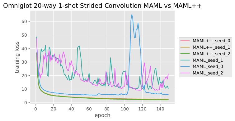 However, we noted that changes as simple as using strided
convolutions or adding more layers into the network, rendered it very unstable (as supported by the training loss oscillations in figure 2), in the sense that the train loss itself oscillated instead of smoothly being minimized.
However, we noted that changes as simple as using strided
convolutions or adding more layers into the network, rendered it very unstable (as supported by the training loss oscillations in figure 2), in the sense that the train loss itself oscillated instead of smoothly being minimized.
This effectively meant that the model required far longer to train, and the model’s final generalization performance was potentially lower than what it could have been if the model was more stable.
So, why is it unstable?
One of the most frequent sources for instability in deep neural networks, are gradient degradation problems, that is, vanishing and exploding gradients. Furthermore, the signature of this instability was eerily similar to some experiments I’d done in the past with extremely deep networks.
In this instance we have a standard 4-layer convolutional network followed by a single linear layer, unrolled for 5 times. Since the inference graph that backprop has to traverse is effectively composed by a cascade of 25 layers, with no skip-connections, then gradient degradation could make sense. In addition, between each model update operation we also compute derivatives with respect to gradient computation itself, which introduces additional backpropagation operations that can cause gradients to degrade even further.
Ok, fair enough, are there any other symptoms or interesting model behaviour patterns that might shed additional light?
The instability disappears when we use 1-3 inner loop steps, and re-appears when we use 4-5 steps. This indicates that the depth of the computational graph has a direct effect on instability. Furthermore, a brief inspection of gradient summary statistics indicated that in 5-step models the gradients returning to the parameter initialization model appear to have very high max values and very low min values (close to 0).
Solution
Let’s assume that gradient degradation is indeed the problem, how can we solve it?
Adding skip-connections that connect the various iterations of the model is probably not a very good idea, as that might introduce additional gradient computational overheads and make things slower and more complex. Thus, another possible route is to introduce explicit per-step gradients. If the model received gradients immediately after each inner-loop step, then the gradient degradation problem could be decreased significantly. At the same time we could add the implicit gradients that the original MAML loss is using, so our model remains focused on the main goal as well. Explicit gradients can be introduced by computing the target set loss after every inner loop update, then computing a weighted average of the per-step losses to be the optimization loss. The weight for each step’s loss can be annealed such that initially all steps have equal importance, and as the experiment progresses the last step’s loss becomes the most important one, thus slowly transitioning to the original MAML loss. This is important to do, to ensure that the model attempts to minimize the last step’s loss the most by the end of the experiment. This ensures that the additional update steps are utilized as much as possible.
After implementing the proposed method, we observed that the training performance stabilized, thus improving convergence speed and having a minor positive impact on the final generalization performance
The next paragraph explains how MAML with multi-step loss works. This is the second most important paragraph (out of two) in this blog-post. So before proceeding, take a sip from your beverage and take a moment to fix your posture. Once you feel ready, march on, to a crash course on MAML MSL.
Figure 3 illustrates how multi step loss optimization works. So, the only difference between MAML and MAML with MSL, is that after each inner loop update step \(\theta_{i} = \theta_{i-1} - \alpha \nabla_{\theta_{i-1}}L^S_{i-1}\), we compute the target set loss using the current weights \(\theta_{i}\), instead of directly proceeding to execute yet another update with respect to the support set. After \(N\) steps have been completed, and \(N\) target set losses (one for each parameter state after each update step) have been obtained. We take a weighted sum of these losses \(L^{T}_{0..N} = \sum^{N}_{N=0} w_iL^T_i\), and optimize the outer loop parameters \(\theta\) using the combined loss.
Figure 3 MAML MSL Computation Graph

\(w\) here is a \(N\) dimensional importance weight vector, that indicates the importance of each steps loss towards the overall loss. During early training, all losses have about equal importance, and as training progresses, the importance weights are annealed, such that earlier step losses have increasingly lower importance, and the \(N^{th}\) step loss has increasingly higher importance assigned to it. As a result the model slowly transitions into the original MAML loss, whilst making sure that the gradients received at each update step, are cleaner and less probable to cause gradient degradation issues.
Well done. This is all one needs to understand to be able to implement and use the multi-step loss technique (assuming a good level of skill in deep learning frameworks).
Omniglot 20-way Few-Shot Classification Results Table
| Approach | 1-shot | 5-shot |
| Siamese Nets | 88.2% | 97.0% |
| Matching Nets | 93.8% | 98.5% |
| Neural Statistician | 93.2% | 98.1% |
| Memory Mod. | 95.0% | 98.6% |
| Meta-SGD | 95.93\(\pm\)0.38% | 98.97\(\pm\)0.19% |
| Meta-Networks | 97.00% | - |
| MAML (original) | 95.8\(\pm\)0.3% | 98.9\(\pm\)0.2% |
| MAML (local replication) | 91.27\(\pm\)1.07% | 98.78% |
| MAML + MSL | 91.53\(\pm\)0.69% | - |
| MAML + LSLR | 95.77\(\pm\)0.38% | - |
| MAML + BNWB + BNRS | 95.35\(\pm\)0.23% | - |
| MAML++ | 97.65\(\pm\)0.05% | 99.33\(\pm\)0.03% |
Mini-Imagenet 5-way Few-Shot Classification Results Table
| Inner Steps | Accuracy | ||
| 1-shot | 5-shot | ||
| Matching Nets | - | 43.56% | 55.31% |
| Meta-SGD | 1 | 50.47\(\pm\)1.87% | 64.03\(\pm\)0.94% |
| Meta-Networks | - | 49.21% | - |
| MAML (original paper) | 5 | 48.70\(\pm\)1.84% | 63.11\(\pm\)0.92% |
| MAML (local reproduction) | 5 | 48.64% | 64.78% |
| MAML++ | 1 | 51.05\(\pm\)0.31% | - |
| MAML++ | 2 | 51.49\(\pm\)0.25% | - |
| MAML++ | 3 | 51.11\(\pm\)0.11% | - |
| MAML++ | 4 | 51.65\(\pm\)0.34% | - |
| MAML++ | 5 | 52.40\(\pm\)1.13% | 67.15\(\pm\)0.26% |
Furthermore, tables 1 and 2 showcase the relative performance of the two systems.
Objectives achieved by MSL:
- Improve stability of MAML
Step-by-step Batch Normalization for Meta-Learning (BNWB + BNRS)
Problem
In the original MAML paper, the authors implemented batch-normalization without storing any running statistics, and instead using the batch statistics to normalize the activations. Doing so, makes the optimization landscape of learning the betas and gammas far more complex, as we are now effectively sharing the parameters across all possible means and standard deviations that the millions of mini-batches will have. Furthermore, the mean and standard deviation used for normalization are very far from the true mean and standard deviation which as a consequence reduces the generalization performance and convergence speed.
So one might ask, why would they not use standard batch-normalization with stored statistics?
The answer, is in fact, simpler than you might think. After running numerous experiments using standard batch normalization, I found out that it simply did not work. Furthermore, the authors chose to only learn betas, whilst keeping gammas stationary at some default value. Again this practice seems counter-intuitive. And again, the reason is that it won’t work otherwise. I found this fact perplexing.
Solution
Why would one of the most powerful, well-tested and highly reliable normalization layers fail to work in this instance?
Well, after sleeping on it, I had a potential answer to this, and again, it is simpler than one might think. As most problems in science, this one was also stemming from a wrongly placed assumption. We were assuming that the initialization model and all it’s updated iterations had in fact, similar feature-distributions. This assumption, effectively means that we considered models that have been updated multiple times (within the inner loop optimization), as being the same model. Obviously this assumption is far from correct. Especially in the case of MAML, where we are literally learning fast-adapting networks, which in other words, causes the model to quickly change as much as possible to learn a new task. Fixing this issue was as simple as learning per-step batch normalization betas and gammas, as well as storing separate statistics for each of the model’s iterations after each update.
Once these simple changes were made, batch normalization improve the convergence speed and generalization performance substantially. Tables 1 and tables 2 showcase the improvements.
Objectives achieved by BNRS + BNWB:
- Improve convergence speed of MAML
- Improve generalization performance of MAML
Per-Layer Per-Step Learnable Learning Rates (LSLR)
Problem
Selecting an inner loop learning rate can be an arduous process, requiring significant amounts of GPU hours. However, since MAML is framed within a meta-learning setting. One can choose to learn the inner loop learning rates as part of the optimization process. Thus not only ensuring that the inner loop learning rates will perform very well but also reducing the computational power needed to find a very good learning rates. In fact, allowing the network to learn its own inner loop’s learning rate, opens the door to new possibilities. In a recent paper by Li et al[], called Meta-SGD, the authors propose learning one learning rate and direction for each parameter in the network. The results they showcase are state of the art. However, learning one learning rate for each parameter is very expensive memory-wise and computation-wise. Furthermore, in a multi-step setup, one could also learn a learning rate and direction for each update step.
Solution
In an attempt to improve the expressivity of the system whilst keeping the memory and computational expenses similar to MAML, we instead propose learning per-layer, per-step learning rates and directions. What this effectively means, is that we’ll allow the network to learn it’s own learning rate scheduler over the N inner loop steps, whilst allowing the network to learn different learning rates for different layers, thus allowing the network to keep some layers pretty much identical to the initialization, for some others learn with much higher learning rates, and even allow negative learning to take place. By negative learning we mean, taking update steps with negative learning rates. One can refer to that as forgetting, but we think that the term forgetting is not precise. More than likely, MAML learns to model how gradients at specific parameters/layers/time-steps influence future gradients, implicitly as part of training. Thus, by allowing the network to learn its own learning rates for each step and layer, we effectively add more expressivity and thus freedom on how it can go about learning things. Perhaps, most learning rate choices (even negative ones) are only there to steer current and future gradients, to the right direction.
Tables 1 and 2 showcase the effect of LSLR on MAML. One can clearly see that the generalization performance has increased. From inspecting the figures we can also see that convergence speed was increased in a similar manner to how step-by-step batch norm improved the system.
Targets achieved by LSLR:
- Improve convergence speed of MAML
- Improve generalization performance of MAML
Step by Step MAML / MAML++:
The next step was to combine all methods. In addition to the previously mentioned methods, we trained the model using the Adam optimizer with lr = 0.001, b1 = 0.9, b2=0.99 cosine annealing the learning rate down to 0.00001 over 150 epochs, each consisting of 500 outer loop updates. Table [1] shows the results of the approach, showcasing that the combined approaches allow for even further improvement in generalization performance and convergence speed, all whilst being highly stable and robust.
Can we learn anything from the learned learning rates? (Meta-meta-learning?)
One of the most important premises of meta-learning is automation of research in a way. The learned per-step per-layer learning rates represent an automatically learned solution. Since these learning rates work with the learned parameter initialization, they are not directly applicable to standard deep neural network training, however, they may provide interesting hints/insights into strong ways of learning to few-shot learn. For that reason, in this section we investigate the learned learning rates. Below we provide an interactive plot showcasing the learned learning rates, in an unrolled manner. Each data point showcases the learning rate (y-axis) of a particular layer (x-axis). Furthermore, by changing the epoch number one can see the state of the learned learning rates at that particular epoch. Each colour indicates a different seed/independent run.
Interactive chart 1: Omniglot 20-way 1-shot
Chart initializes at the per-seed best validation model epoch.
In the Omniglot 20-way 1-shot task the system chose to assign very high learning rates to the last convolutional layer’s weights, whereas earlier layers are assigned very small, almost null learning rates in all steps but the last. It appears that the learning rate magnitudes can be grouped into very high learning rates (steps 1 and 3), medium learning rates (step 2 and 4) and low learning rates (step 5). It is almost as if the network is trying to start with very aggressive optimization and then at the last step, gracefully finish its inner loop optimization without overfitting. Another interesting observation here, is the usage of negative learning rates. Earlier layers in the network are more likely to be set to a negative learning rate. It might just be that the network is trying to steer gradients towards the right direction such that future gradients take it to the right target. Or perhaps the network is using forgetting as a means to learn new concepts more efficiently (starting from blank slate?). Finally, it appears that even though earlier layers learned overall much lower magnitude learning rates, step 5 learning rates appear to be about equal across all convolutional layers, which might indicate that the last step is where most of the early layer fine-tuning happens. This might be the case because it is easier for the network to predict the effects of gradients after 1 step, rather than 3-4 steps for example. If the network started tuning all of its layers aggressively from the beginning, then it would have a harder time predicting how it would influence future gradient updates. So by setting most learning rates close to zero, it effectively reduces the number of gradients it has to model, in order to do well in its across-task learning.
Earlier layers might also require less fine tuning because low-level filters generalize well across the board, whereas deeper layer filters are not as generalizable and need more tuning. This phenomenon, of earlier layers being more generalizable has been observed before in the deep learning literature. It might also tie in with the fact that removing or degrading earlier layers causes a deep neural network to receive massive degradation in its performance, whereas removing deeper layers has much less influence on the system’s performance. Perhaps another reason the system here chose to keep earlier layers stationary is to prevent such catastrophic performance degradation from occurring.
Interactive chart 2: Omniglot 20-way 5-shot
Chart initializes at the per-seed best validation model epoch.
In the Omniglot 20-way 5-shot task, the learned learning rates follow similar trends to the 20-way 1-shot tasks. However, the overall learning-rate magnitudes are higher and seem to decrease linearly. This is probably due to the availability of additional samples per class, which generate better gradients that have increased generalization performance. Since generalization performance is less of an issue, the system chooses to use a smoother learning rate schedule instead of a (more secure) contrastive one. Furthermore, it appears that in the 20-way 5-shot task, the system has assigned higher learning rates at earlier layers (compared to the respective layers in the 20-way 1-shot task). Perhaps, in a 1-shot task the network prefers to minimize inner loop update magnitudes as much as possible, since the risk of overfitting is much higher. Whereas, in the 20-way 5-shot task, the availability of additional data reduces the risk of overfitting and thus the network chooses to increase inner loop learning. Another possible interpretation is that the future time-step gradients are easier to predict when more samples are available, thus the network is more confident at how the final state will look like, hence it can schedule to higher magnitude gradient updates, with much lower risk of overfitting.
Interactive chart 3: Mini-imagenet 5-way 1-shot
Chart initializes at the per-seed best validation model epoch.
In mini-imagenet 5-way 1-shot, it appears that the learning rate scheduler strategy is very different than those of Omniglot. The network chooses to use approximately equal magnitude learning rates for the first 4 steps, before significantly increasing the magnitudes in the very last step. This comes in direct contrast with the Omniglot tasks, and it might indicate that there is less overfitting happening in the support set, hence choosing to maximize learning as much as possible by using larger magnitude learning rates across all steps. It’s also worth noting that layer 1 is assigned basically close to zero learning rates, thus effectively showing that early layers generalize well across tasks, with no added learning required. Another difference from Omniglot learned learning rates is that the linear layer biases are set to very high learning rates, thus showing that more energy needs to be expended to learn the most generalizable biases at each step. This makes intuitive sense as the class contents are far more diverse and complicated than Omniglot, thus requiring more tuning on the linear biases side of things. Some similarities with the Omniglot learned learning rates is that, the last convolutional layer is assigned the highest magnitude learning rate consistently, again showcasing that later layer features do not generalize as well and need more fine-tuning.
Some additional interesting observations is that it appears that across seeds, often learning rates can be reflections of each other, showcasing that the direction might be very dependant on the parameter initializations learned, however the magnitudes are task dependent and appear to be consistently at very similar magnitudes across seeds.
Interactive chart 4: Mini-imagenet 5-way 5-shot
Chart initializes at the per-seed best validation model epoch.
In mini-imagenet 5-way 5-shot, the learned learning rates are very similar to the 5-way 1-shot learning rates, but with a twist. Since the system is given more data-points for each class, it appears that the system chooses to decrease the learning rates at the last step substantially, to gracefully finish learning the new task, potentially to avoid overfitting or to reach a more “predictable” state, which might also be more generalizable.
One should also keep in mind, that the learning rates learned, are to be used with the jointly learned parameter initialization. In other words, the learned learning rates serve as additional modelling capacity that allows the network to reach a very generalizable state for a target task faster, and as the above charts show, with far more flexible inner loop learning. Since the network in most parts chooses to set a very low learning rate, whilst at other key parts chooses to set a very high learning rate, one could say that the model learned is far simpler and only updates its weights only towards the necessary directions, keeping as many layers stationary as possible. This might allow the network to learn a simpler parameter initialization, one that is not updated at all layers, hence one that is easier to arrive to. As a result, the system can learn a simpler parameter initialization, which enhanced by the flexible learning rates, can achieve stronger generalization performance. Effectively the flexible learning rates act as an Occams Razor of sorts, which keeps the network as simple as possible, but not simpler than that.
Why did you spend all this time just to improve a very specific meta-learning framework like MAML?
We weren’t really trying to improve MAML in particular. We were trying to improve end-to-end differentiable gradient-based meta-learning that utilizes inner loop optimization to learn at inference time. The potential of this particular type of meta-learning is immense, as it provides very sample-efficient meta-learning (when compared to RL and GA counterparts). MAML is a high performance and light-weight instance of gradient-based meta-learning, which makes it an ideal base on which one can build more complicated models. However, after attempting to use MAML we noticed many of its shortcomings (which are almost definitely present in other gradient-based meta-learning systems). Thus solving the problems that MAML has exposed is vital, not only for MAML itself, but for meta-learning as a whole. Once those problems are solved, one can begin to tap the potential of gradient-based meta-learning by building more interesting and complicated systems on top of existing gradient-based meta-learning frameworks (such as MAML).
Conclusion
The potential of meta-learning in solving hard problems is immense and at the current stage completely untapped. For the first time ever, we have the compute and software required to train very complicated meta-learning systems that can learn their own internal inference blocks. In this blog-post we demonstrated how one can stabilize and improve a very elegant and powerful such system, called MAML. In our attempts to improve it, we introduced a batch normalization layer adapted for meta-learning, a new optimization loss and a way to learn per-layer per-step learning rates. The resulting learned learning rates provided a lot of insight into how a good few-shot learning system can be built, and made for very interesting and information dense visualizations that can provide further information into how we can build even better meta-learning systems. There is a lot more to be discussed about that aspect, but more of that in our next blog post.
Thanks for reading my blog. That’s it for this time. See you again in the future.